Table of contents
1 Introduction
1.1 Wise man
In the Latin name for modern humans, Homo sapiens, which literally translates to “wise man”, we can see the importance we place on our intelligence and on our abilities such as reasoning, speech, logical problem-solving, and consciousness. We often consider intelligence to be defining factor that sets us apart from other species. It shapes our self-perception but we do not understand it yet. I believe that attempting to define certain scientific disciplines and fields is a rather ungrateful task, and for that reason, I will not engage in an in-depth analysis or explanation of the field of artificial intelligence itself. In its simplest form, the definition of this research area could be described as the study and creation of intelligent entities. The very understanding of intelligence, and what makes an entity intelligent, leads to highly diverse classifications and approaches in attempts to create such entities. Alan Turing proposed the Turing Test in 1950 as a way to determine whether a machine is intelligent. Turing established that a computer could be considered intelligent if, through written interaction with a human, it could convince that person that they are communicating with another human rather than a machine. To make this possible, the computer would need to possess the following abilities: natural language processing, knowledge representation, automated reasoning, and the ability to learn from new data, which would allow it to adapt to new circumstances.
1.2 Natural language processing
Natural language processing is a field of artificial intelligence that deals with the tasks of understanding and generating natural language by computers. Since language is a human abstraction that we created to describe the world around us, it seems like it holds the potential to serve as a tool for building very powerful and useful models. This can be glimpsed through current large language models, which demonstrate the ability to learn highly complex patterns and generate coherent, human-like text. Their strength lies in their capacity to grasp the deep structure embedded in language - a structure that mirrors and describes the logic and relationships present in the real world. This is the main reason why such models can answer our questions, summarize texts, translate between different languages correctly, and more without being explicitly trained to perform some of those tasks.
1.3 Machine Learning
The modern field of natural language processing relies on machine learning algorithms. Machine learning is a subfield of artificial intelligence that focuses on creating algorithms that enable computers to learn from data without the need for explicit programming. The foundation for the development of this field lies in inductive reasoning, which has long been studied in mathematics and deals with drawing general conclusions based on a limited set of data.
1.4 History of langauge modeling
Natural language processing represents one of the essential fields of artificial intelligence. The algorithms developed within this field aim to enable machines to understand and generate text in a human-like way. A statistical language model represents a function that assigns a probability of occurrence to each sequence of words. Formally, a language model is a joint probability distribution:
Let's consider a small example:
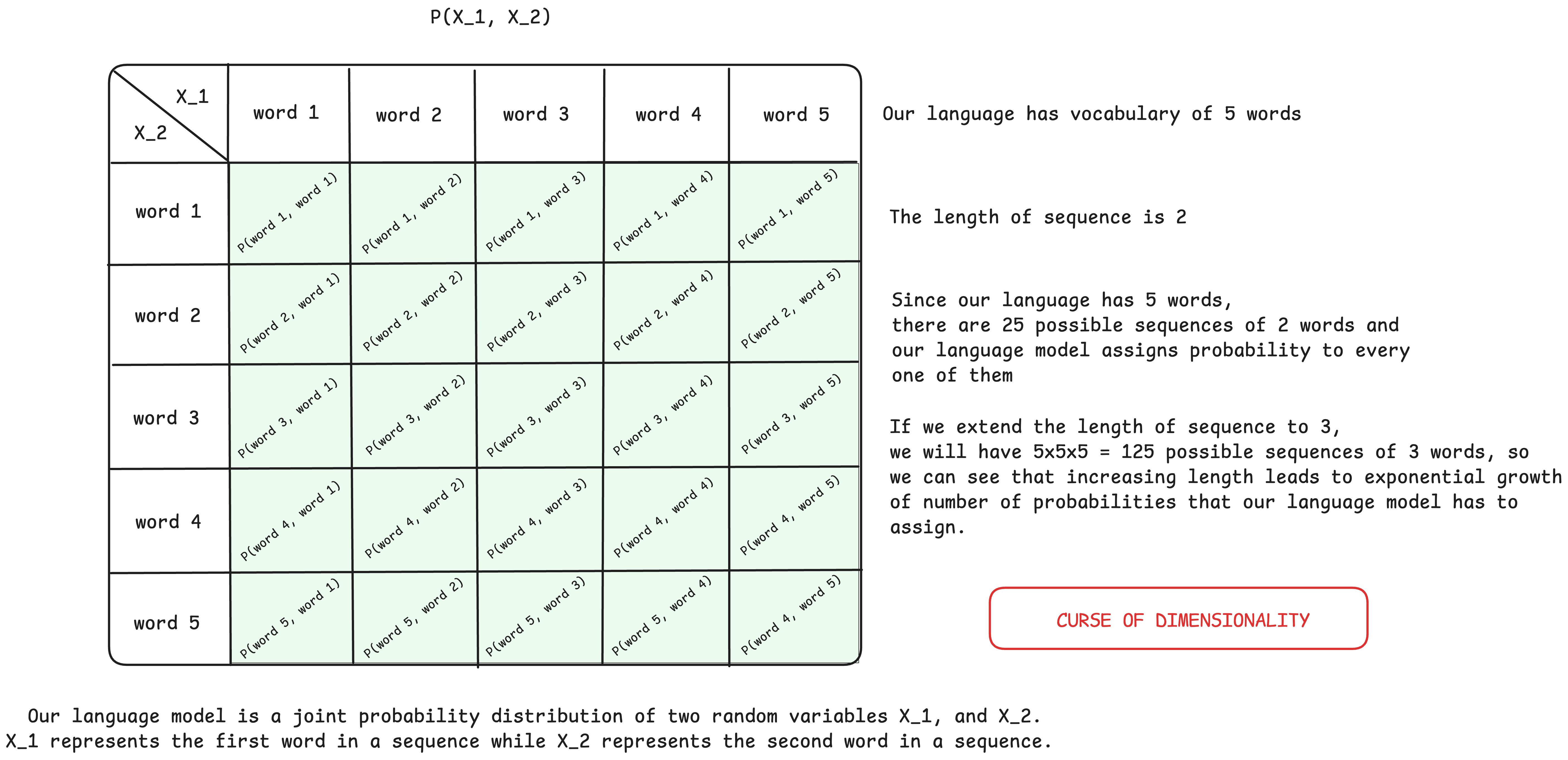
Figure 1: Tabular representation of the probability distribution of word sequences.
Knowing the joint probability distribution of word sequences allows predicting the most likely next word in the sequence. By the definition of conditional probability we get:
The problem arises because the joint distribution of a word sequence is very difficult to model directly because the number of possible sequences grows exponentially with the increase in the length of the sequence, as well as the amount of data that is necessary for a reliable estimation of probabilities. This problem can be simplified by factoring the joint probability distribution into smaller units using the chain rule of probability:
To further facilitate modeling, long-popular models, n-grams, estimate the probability of the next word in a sequence by introducing an independence assumption. This is called the Markov assumption, and such models imply that the word that is currently being predicted does not depend on the complete sequence of words that precede it, but only on the surrounding context of a fixed length (Rosenfeld, 2000). From there we get the following equation:
N-grams consider context of n-1 words, so models that take a single-word context are called bigrams, while models that take a two-word context are called trigrams. Models based on n-grams have been very popular for a long time, but they suffer from several problems, the main ones being the curse of dimensionality, poor generalization ability, i.e. poor performance on data that differs from the training set, as well as the inability to understand dependencies between words in a sentence. In order to solve these problems, researchers have created techniques such as backoff, interpolation and smoothing, but they are still not enough to overcome the mentioned challenges.
1.5 Standing on the shoulders of giants
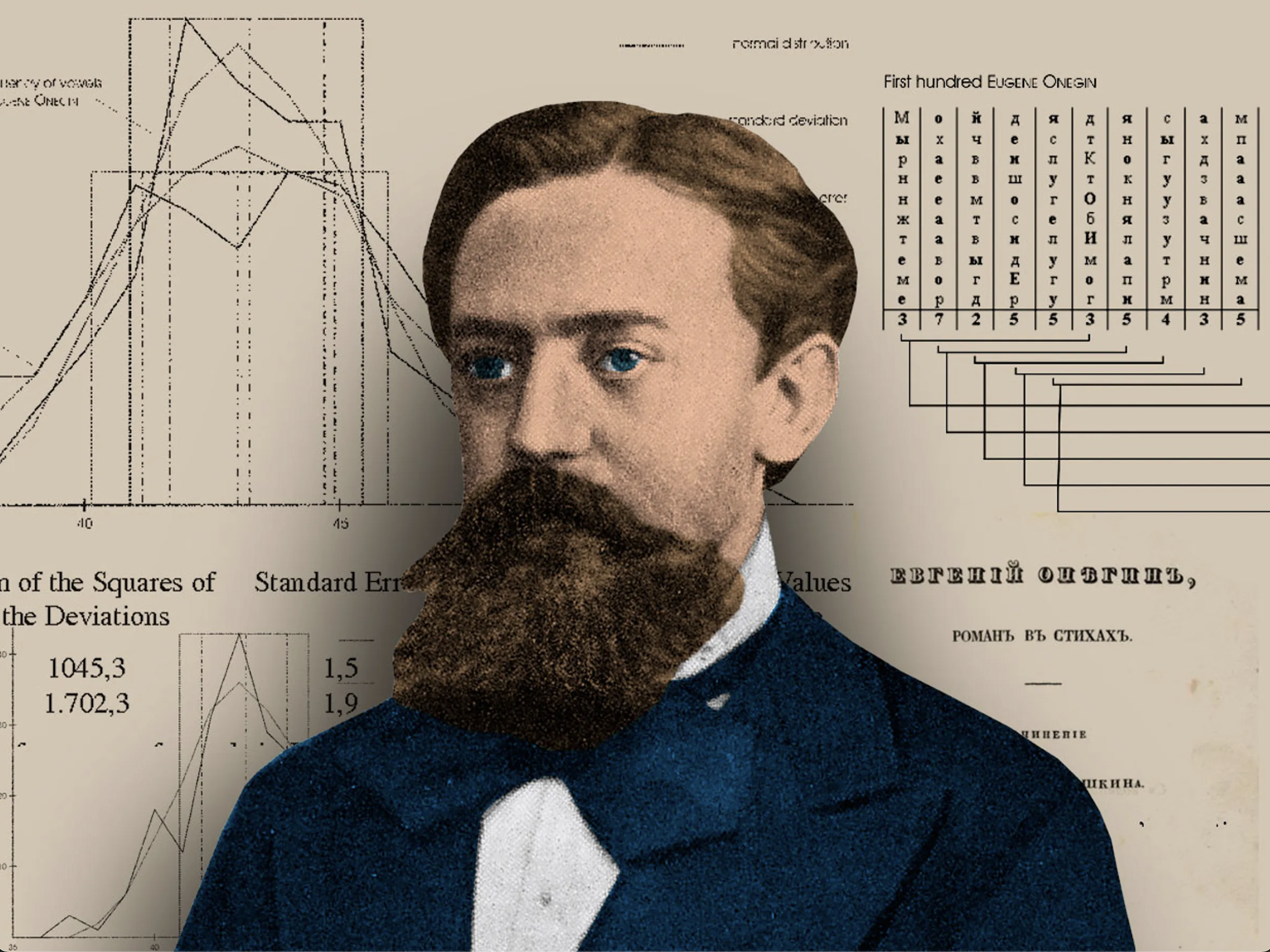
Figure 2: Russian mathematician Andrey Andreyevich Markov in front of his statistical analyses of Alexander Pushkin’s novel, Eugene Onegin. Taken from https://spectrum.ieee.org/andrey-markov-and-claude-shannon-built-the-first-language-generation-models
It can be said that the foundations of language modeling were laid by the Russian mathematician Andrei Markov, who examined the fundamental mathematical structure present in language by observing the text of Pushkin’s famous work, Eugene Onegin. He took the first 20,000 letters of this work, removed punctuation marks and spaces, and then observed the overall probabilities of consonants and vowels.
He proved the existence of dependence and structure in language by observing pairs of vowels and consonants, realizing that the probabilities of their occurrence were not independent, but rather dependent on the symbol preceding them. Markov developed a theory and framework that allows us to calculate the probability of a sequence of random events where a future event depends solely on the current one.
His discovery represented a significant contribution to probability theory, which until then had largely relied on the necessity of considering mutually independent events. You can read the translation of his original work here.

Figure 3: Portrait of Claude Shannon
The idea of structure being present in language was further accepted and expanded upon by Claude Shannon, who formulated the first serious statistical model of the English language and simultaneously established the field of information theory. He defined the concepts of information and entropy, which continue to play a crucial role in training various types of machine learning models, including Large Language Models. You can find more information in his paper called A Mathematical Theory of Communication.
1.6 Models based on neural networks
The foundations of language models based on neural networks were laid by Yoshua Bengio (2003) who introduced the concept of neural networks that use continuous vector representations of words. In this way, Bengio enabled language modeling, i.e. prediction of the next token by using a significantly larger amount of information compared to the use of discrete representations that only carry information about word identity, but not about meaning and semantics. A great contribution was also made in the field of generalization because due to the presence of semantics in the vector representations of words, the model learned to differentiate between semantically similar and semantically different words. This allowed the model to distribute probability to semantically similar sequences even when one did not appear in the training corpus.
Let's see the comparison of bigram and neural network based model through this small example:
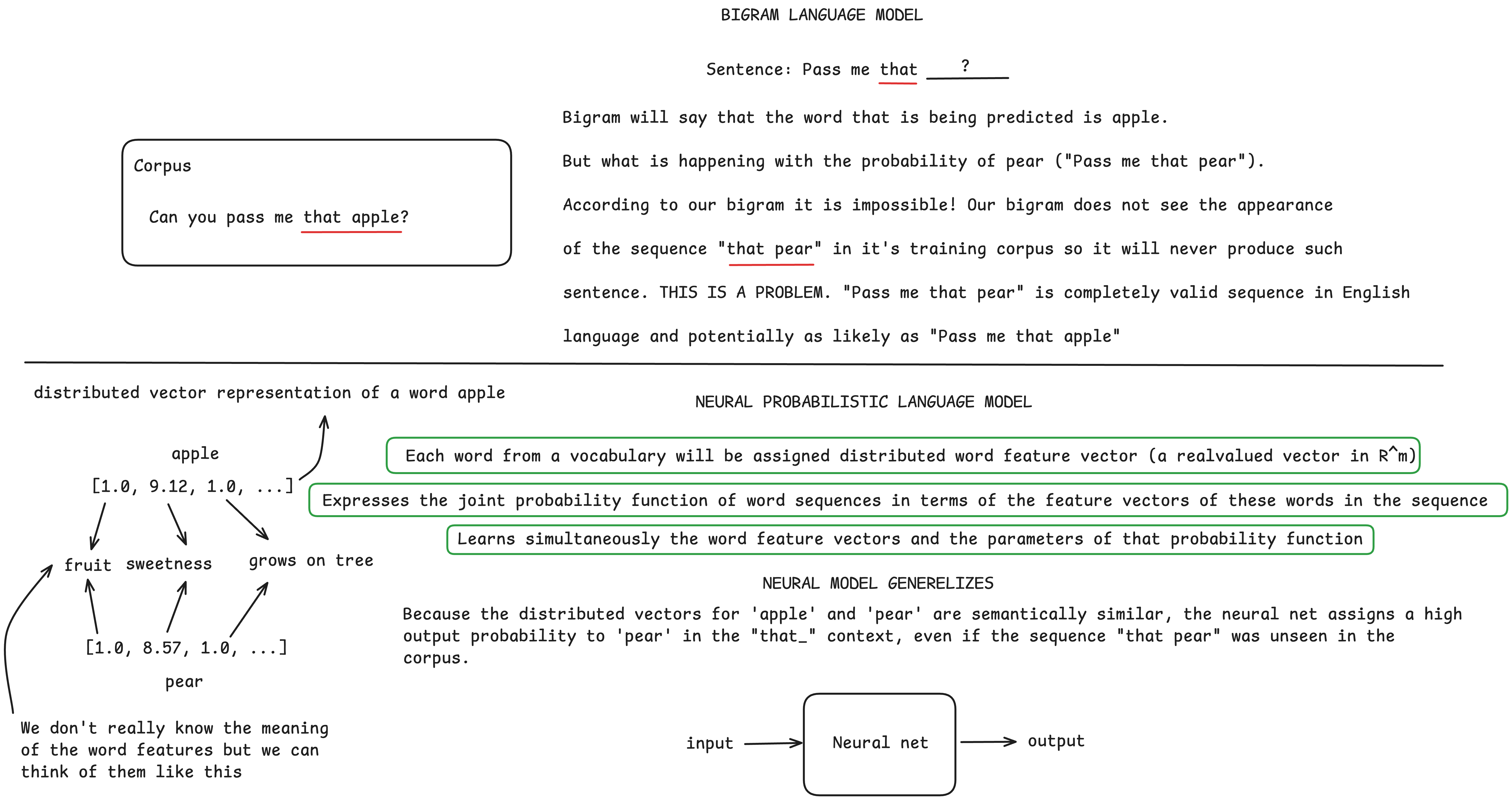
Figure 4: Comparison of bigram and neural network-based language models.
Bengio et al. (2003) used a feedforward neural network in their work, while Mikolov et al. (2010) were the first to use a recurrent neural network for language modeling purposes.
Mikolov et al. (2013) brought big changes to the world of natural language processing with the publication of their word2vec model. They used neural networks and a large corpus of text to generate vector representations of words that retain the semantics that are present in the language. In contrast to Bengio et al. (2003), they did not train a full language model; instead, they learned only word feature vectors. Representations created in this way enabled the transfer of knowledge within the domain of natural language processing, making it possible to train models using word2vec word vectors and achieve better results on various NLP tasks, including natural language modeling.
Although word2vec brought significant improvements, the problem of polysemy was present. For a specific word from the vocabulary, word2vec would produce a unique static vector representation, however, one word can have several different meanings depending on the context in which it is found. Peters et al. (2018) published a paper where they showed the importance of contextualized representations of words that actually dynamically adapt, depending on the context in which the word is found. They used the values of the hidden layers of a pretrained language model based on a bidirectional recurrent neural network architecture to obtain context-dependent vector representations of words that can then be used to improve performance on other natural language processing tasks.
2 Transformer
Vaswani et al. (2017) present a transformer architecture, created for the needs of machine translation, very suitable for parallelization on GPUs and training on a large amounts of data. The Transformer completely forgoes recurrent units and relies entirely on the attention mechanism, retaining the encoder and decoder components that were standard parts of the dominant sequence translation models of the period. This architecture is the foundation of most modern large language models.
Figure 5: Architecture of the transformer model. Adapted from Vaswani et al. (2017).
2.1 Encoder
The task of the encoder is to convert the original input sequence into contextualized vector representations that can be used by the decoder to generate text. The encoder part of the original transformer consists of 6 consecutive blocks, each of which is composed of an attention module and a multilayer perceptron (Vaswani et al., 2017). The attention module and multilayer perceptron are followed by residual connection (He et al., 2015), and layer normalization (Ba et al., 2016).
Most modern models used for the task of causal language modeling actually omit the encoder part and rely only on the decoder part of the transformer. However, there are also models that exclusively rely on the encoder part of the transformer, such as BERT (Devlin et al., 2018) and RoBERTa (Liu et al., 2019). Due to the bidirectional attention applied in the encoder module, such models are very good for text classification tasks, recognition of named entities or generation of semantically rich vector representations that can later be used for information extraction.
2.2 Decoder
The decoder part of the transformer consists of 6 consecutive blocks, each block containing an attention module and a multilayer perceptron just like the encoder, but the difference is that the decoder contains an additional masked attention module (Vaswani et al., 2017). The authors of the paper called this module masked self-attention, and its role is to allow paying attention only to previously generated tokens, preventing insight into future positions. Residual connection and normalization layers are retained after each of the listed transformer modules. Models based on the decoder part of the original transformer are suitable for the task of causal language modeling.
2.3 Attention mechanism
A very important moment for the field of natural language processing occurred with the introduction of the attention mechanism created by Bahdanau, Cho, and Bengio (2014), which was originally applied to a recurrent neural network trained for the task of machine translation. Bahdanau, Cho, and Bengio (2014) focused on the problem of understanding dependencies between distant words in a sentence. In the models of the time, the decoder initially generated outputs only based on the last output representation of the encoder, which was not informative enough, and the translation generated by the decoder was often poor.
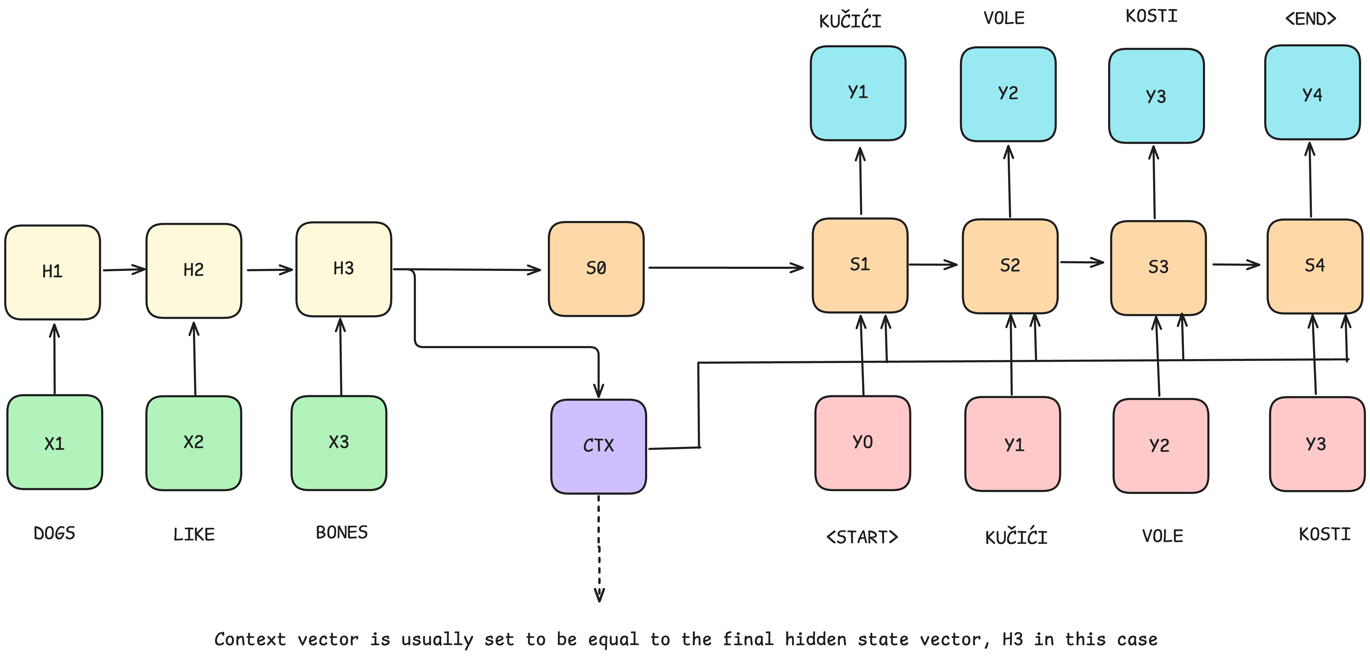
Figure 6: Illustration of the sequence-to-sequence models.
In order to solve this deficiency, Bahdanau et al. (2014) extend the existing encoder-decoder architecture and allow the decoder part to refer to the input sequence, more precisely, to the encoder representations of words from the input sequence, each time before generating the next word. In this way, they managed to solve the need for the model to encode all dependencies from the input sequence into a singular vector representation. The decoder got the ability to choose which words from the input sequence it wants to pay more attention to when generating the next word. They initially called this mechanism alignment.
Figure 7: Representation of attention patterns in the English to French translation task. Each pixel indicates the relevance of the input at position j to generate the output at position i. Brighter pixels indicate more importance. Adapted from Bahdanau, Cho, and Bengio (2014).
Although this mechanism gave improved results on the task of machine translation, especially when it comes to the translation of longer sequences, the problem was that it introduced additional computational complexity because it requires the calculation of the attention strength, i.e. the annotation weights as it was called in the original work, for all words from the output sequence (Bahdanau et al. 2014).
Figure 8: Architecture of the attention mechanism introduced by Bahdanau et al. (2014).
The attention mechanism is the key component of the transformer architecture and forms the foundation of modern large language models. The transformer presented by Vaswani et al. (2017) eliminated recurrent layers, enabling a high level of parallelization. This solved the problem of sequential computation of attention weights. In addition to cross-attention, the mechanism where the decoder uses the representations generated by the encoder to produce the most relevant outputs, the authors also introduced a self-attention mechanism that allows words within the same sequence to exchange information and establish mutual relationships. Through this mutual exchange of information between tokens via the attention mechanism, rich context-aware representations are created, providing an excellent basis for numerous tasks in natural language processing, such as language modeling, text classification, named entity recognition, and others.
Figure 9: Illustration of the self-attention mechanism. In the given example, the word making pays attention to the words more and difficult, providing the information that the verb is used in the context of the phrase “making more difficult,” which should be reflected in the vector representations of these words produced by the attention module. Adapted from Vaswani et al. (2017).
It is important to note that the encoder module of the transformer uses a bidirectional self-attention mechanism so that the vector representations of words, on the basis of which translation will be performed (the task the architecture was originally designed for), contain as much contextual information as possible. In contrast, the decoder uses masked self-attention. The reason for using masked self-attention is the causal nature of language modeling. The word, or token, currently being predicted depends only on the tokens that precede it, and not on those that come after it. For this reason, tokens within the masked self-attention module are allowed to look back and establish relationships only with tokens that appear earlier in the sequence.
Figure 10: Self-attention mask that is applied in self-attention module
2.4 Transformer coded
# LEVEL 0 building blocks - For the learning purposes I decided to implement
# the most basic building blocks of Transformer model.
# Keep in mind that some of these are not the optimal implementations
# of these layers and serve for educational purposes (MHA for example).
class LayerNorm(nn.Module):
"""
Class representing layer normalization.
Normalizes input using layer mean and layer variance.
Holds parameters for scaling and shifting that are learned during the training.
It is possible to use nn.LayerNorm instead as it is provided by PyTorch.
"""
def __init__(self, shape, epsilon = 1e-5):
super().__init__()
self.epsilon = epsilon
self.scale = nn.Parameter(torch.ones(shape))
self.shift = nn.Parameter(torch.zeros(shape))
def forward(self, x):
mean = torch.mean(x, dim=-1, keepdim=True)
var = torch.var(x, dim=-1, keepdim=True, unbiased=False)
x_normalized = (x - mean) / torch.sqrt(var + self.epsilon)
return self.scale * x_normalized + self.shift
class Dropout(nn.Module):
"""
Regularization technique used in neural nets in order to prevent overfitting.
Randomly deactivates subset of neurons from the layer with probability p which prevents network to over-relying on any specific subset of neurons (co-adaptation).
Dropout is only applied during the training. During the inference all of the neurons are active.
This implementation uses the inverted dropout that introduces scaling of the activations during training so
expected value of the output during training equals the expected value of the output during inference.
It is possible to use nn.Dropout as it is provided by PyTorch.
"""
def __init__(self, p = 0.5):
super().__init__()
if p < 0 or p > 1:
raise ValueError(f"Dropout probability must be between 0 and 1, but got {p}")
self.p = p # Probability of neuron to be turned off during training
self.keep_probability = 1 - self.p
def forward(self, x):
if self.training:
dropout_mask = torch.bernoulli(torch.empty_like(x), self.keep_probability) # We will create a mask where each element in the tensor will be set to 1 with 1-p probability (neuron stays turned on - keep probability)
# Inverted dropout
# When applying dropout we would like to get E[masked_output] = keep_probability * E[unmasked_output]
# So in order to get the same expectation of outputs during training and inference (where there is no masking) we will scale E[masked_output] by 1/keep_probability
# E[masked_output] / keep_probability = E[unmasked_output]
return (x * dropout_mask) / self.keep_probability
else:
return x
class Linear(nn.Module):
"""
Class that represents the implementation of Linear layer.
This implementation uses Kaiming (He) uniform initialization
is the default weight initialization scheme for nn.Linear and it should work nicely with ReLU activation
It is possible to use nn.Linear instead as it is provided by PyTorch.
"""
def __init__(self, in_features, out_features, bias=True):
super().__init__()
self.in_features = in_features
self.out_features = out_features
self.W = nn.Parameter(torch.empty(out_features, in_features))
if bias:
self.bias = nn.Parameter(torch.empty(out_features))
else:
self.register_parameter("bias", None)
self.reset_parameters()
def reset_parameters(self):
nn.init.kaiming_uniform_(self.W, a=math.sqrt(5))
if self.bias is not None:
nn.init.zeros_(self.bias)
def forward(self, x):
output = x @ self.W.T
if self.bias is not None:
output += self.bias
return output
class Embedding(nn.Module):
"""
Class that represents the Embedding layer.
Essentially it is a table (matrix) that holds word embeddings.
In the very begginging weights (word embeddings) are initialized randomly from Normal distribution with mean = 0 and std = 1,
but get adjusted during the training.
Matrix has the shape of (num_embeddings, embed_dim) - essentially meaning it has vocabulary size rows - each word (token) from vocab gets a row and each row has
embed_dim columns. This represents the dimensionality of singular word (tokene) embedding.
Forward method just performs retreival of the token embeddings associated with indeces that were passed as arguments.
It is possible to use nn.Embedding instead as it is provided by PyTorch.
"""
def __init__(self, num_embeddings, embed_dim):
super().__init__()
self.num_embeddings = num_embeddings
self.embed_dim = embed_dim
self.W = nn.Parameter(torch.empty(self.num_embeddings, self.embed_dim))
self.reset_parameters()
def reset_parameters(self):
torch.nn.init.normal_(self.W)
def forward(self, x):
return self.W[x]
class MultiHeadAttention(nn.Module):
"""
Class that represents the Multi Head Attention mechanism implementation.
It is possible to use nn.MultiheadAttention instead as it is provided by PyTorch.
"""
def __init__(self, config):
super().__init__()
self.config = config
# For the demonstration purposes I will do the follwoing
self.n_heads = self.config['n_heads']
self.embed_dim = self.config['embed_dim']
assert self.embed_dim % self.n_heads == 0, "embed_dim must be divisible by n_heads"
self.head_dim = self.embed_dim // self.n_heads # So we have embed_dim = head_dim * n_heads
self.W_k = Linear(self.embed_dim, self.head_dim * self.n_heads) # These are weights that will be used to obtain all of the keys for all of the heads
self.W_q = Linear(self.embed_dim, self.head_dim * self.n_heads)
self.W_v = Linear(self.embed_dim, self.head_dim * self.n_heads)
self.W_o = Linear(self.embed_dim, self.embed_dim)
def forward(self, q, k, v, mask=None):
batch_size, seq_length, embed_dim = q.shape
Q = self.W_q(q) # (batch_size, seq_length, embed_dim)
K = self.W_k(k) # (batch_size, seq_length, embed_dim)
V = self.W_v(v) # (batch_size, seq_length, embed_dim)
# Now let's reshape these tensors
Q = Q.reshape(batch_size, seq_length, self.n_heads, self.head_dim) # (batch_size, seq_length, n_heads, head_dim)
K = K.reshape(batch_size, seq_length, self.n_heads, self.head_dim)
V = V.reshape(batch_size, seq_length, self.n_heads, self.head_dim)
# And transpose
Q = Q.transpose(1, 2) # (batch_size, n_heads, seq_length, head_dim)
K = K.transpose(1, 2)
V = V.transpose(1, 2)
attn_scores = (Q @ K.transpose(2, 3)) / (self.head_dim ** 0.5) # (batch_size, n_heads, seq_length, seq_length)
if mask is not None:
attn_scores = attn_scores.masked_fill(mask == 0, float("-inf"))
normalized_attn_scores = F.softmax(attn_scores, dim=-1) # (batch_size, n_heads, seq_length, seq_length)
# normalized_attn_weights (batch_size, n_heads, seq_length, seq_length) @ V (batch_size, n_heads, seq_length, head_dim)
# results in y of shape (batch_size, n_heads, seq_length, head_dim)
y = normalized_attn_scores @ V
# Now lets transpose the output tensor so we get tensor of the following dimensions (batch_size, seq_length, n_heads, head_dim)
y = y.transpose(1, 2)
# Now we can concat output from each head and obtain the embedding of original dimenions
# We should make tensor contiguous in memory before reshaping, to avoid issues after transpose
y = y.contiguous().reshape(batch_size, seq_length, embed_dim)
# Finally we just project the output through the linear layer
y = self.W_o(y)
return y
class PositionalEncoding(nn.Module):
"""
Class that represents implementation of sinusoidal encodings that are used
for encoding of positional information in the original Transformer paper.
"""
def __init__(self, config):
super().__init__()
self.config = config
self.register_buffer("pe", self.create_pe_matrix())
self.dropout = Dropout(config['dropout'])
def create_pe_matrix(self):
positional_encoding_matrix = torch.zeros((self.config['max_seq_length'], self.config['embed_dim']))
positions = torch.arange(0, self.config['max_seq_length']).unsqueeze(1)
division_terms = 1 / 10000 ** (torch.arange(0, self.config['embed_dim'], 2) / self.config['embed_dim'])
positional_encoding_matrix[:, 0::2] = torch.sin(positions * division_terms)
positional_encoding_matrix[:, 1::2] = torch.cos(positions * division_terms)
return positional_encoding_matrix
def forward(self, x: torch.Tensor):
batch_size, seq_length, embed_dim = x.shape
# PyTorch will broadcast this automatically since x and pe[:seq_length] have the same size for 2 dimensions
return self.dropout(x + self.pe[:seq_length])
# LEVEL 1 building blocks
class MLP(nn.Module):
"""
Class representing Point Wise Feed Forward network described in the Transformer paper.
Some versions also use dropout in MLP, but the original paper did not mention it here so I decided not to use it.
"""
def __init__(self, config: dict):
super().__init__()
self.config = config
self.W_1 = Linear(self.config['embed_dim'], self.config['dff'])
self.W_2 = Linear(self.config['dff'], self.config['embed_dim'])
def forward(self, x: torch.Tensor):
return self.W_2(F.relu(self.W_1(x)))
class ScaledEmbedding(nn.Module):
"""
Class that represents scaled embeddings used in the original transformer
"""
def __init__(self, num_embeddings, embed_dim):
super().__init__()
self.embeddings_table = Embedding(num_embeddings, embed_dim)
self.embed_dim = embed_dim
def forward(self, x):
embeddings = self.embeddings_table(x) # (batch_size, seq_length, embed_dim)
return embeddings * math.sqrt(self.embed_dim)
# LEVEL 2 building blocks
class DecoderBlock(nn.Module):
def __init__(self, config):
super().__init__()
self.config = config
self.masked_multihead_attention = MultiHeadAttention(self.config) # masked self-attention
self.norm1 = LayerNorm(self.config['embed_dim'])
self.cross_attention = MultiHeadAttention(self.config)
self.norm2 = LayerNorm(self.config['embed_dim'])
self.pointwise_feed_forward = MLP(self.config)
self.norm3 = LayerNorm(self.config['embed_dim'])
self.dropout = Dropout(self.config['dropout'])
def forward(self, x, enc_outputs, mask):
sublayer_1 = self.norm1(x + self.dropout(self.masked_multihead_attention(x, x, x, mask)))
sublayer_2 = self.norm2(sublayer_1 + self.dropout(self.cross_attention(sublayer_1, enc_outputs, enc_outputs)))
sublayer_3 = self.norm3(sublayer_2 + self.dropout(self.pointwise_feed_forward(sublayer_2)))
return sublayer_3
class EncoderBlock(nn.Module):
def __init__(self, config):
super().__init__()
self.config = config
self.multihead_attention = MultiHeadAttention(self.config)
self.norm1 = LayerNorm(self.config['embed_dim'])
self.pointwise_feed_forward = MLP(self.config)
self.norm2 = LayerNorm(self.config['embed_dim'])
self.dropout = Dropout(self.config['dropout'])
def forward(self, x):
sublayer_1 = self.norm1(x + self.dropout(self.multihead_attention(x, x, x))) # Add encoder mask
sublayer_2 = self.norm2(sublayer_1 + self.dropout(self.pointwise_feed_forward(sublayer_1)))
return sublayer_2
# LEVEL 3 the architecture
class Transformer(nn.Module):
"""
The core class that represents the architecture of the model.
"""
def __init__(self, config):
super().__init__()
self.config = config
self.encoder_embedding_layer = ScaledEmbedding(self.config["enc_vocab_size"], self.config["embed_dim"])
self.decoder_embedding_layer = ScaledEmbedding(self.config["dec_vocab_size"], self.config["embed_dim"])
self.enc_positional_encoding_layer = PositionalEncoding(self.config)
self.dec_positional_encoding_layer = PositionalEncoding(self.config)
self.encoder = nn.ModuleList([EncoderBlock(self.config) for _ in range(self.config["n_layers"])])
self.decoder = nn.ModuleList([DecoderBlock(self.config) for _ in range(self.config["n_layers"])])
self.out = Linear(self.config["embed_dim"], self.config["dec_vocab_size"])
def generate_mask(self, dec_idx):
batch_size, seq_length = dec_idx.shape
mask = torch.tril(torch.ones(seq_length, seq_length, device=dec_idx.device)).view(1, 1, seq_length, seq_length)
return mask
def forward(self, enc_idx, dec_idx):
# enc_idx (batch_size x seq_length)
# [[12, 237, 273]] -> dummy example of idx where batch size is one (meaning one sequence) and seq_length is 3, this means that our sequence consists of 3 tokens and we can see their indeces
batch_size, seq_length = enc_idx.shape
# Mask generation
dec_mask = self.generate_mask(dec_idx)
# ENCODER STAGE
enc_representations = self.encoder_embedding_layer(enc_idx)
enc_representations = self.enc_positional_encoding_layer(enc_representations)
enc_outputs = enc_representations
for layer in self.encoder:
enc_outputs = layer(enc_outputs)
# DECODER STAGE
dec_representations = self.decoder_embedding_layer(dec_idx)
dec_representations = self.dec_positional_encoding_layer(dec_representations)
dec_outputs = dec_representations
for layer in self.decoder:
dec_outputs = layer(dec_outputs, enc_outputs, dec_mask)
output = self.out(dec_outputs) # (batch, dec_seq_len, dec_vocab)
return output
3 Large Language Models
In order to better understand Large Languge Models this section will go over 4 popular LLMs and explore their architectures.
3.1 GPT 2
Radford et al. (2018) presented the first GPT model (Generative pre-trained transformer) that used only the decoder part of the original transformer architecture.
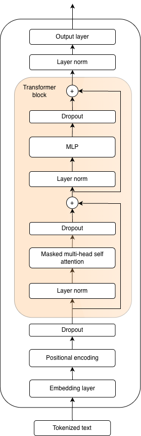
Figure 11: Architecture of the GPT 2 model.
They initially pre-trained the model on a large corpus of text and then fine-tuned it for specific tasks.
The following year, Radford et al. (2019) published GPT-2. Through their work, they demonstrate that sufficiently large models can solve tasks for which they are not explicitly trained.
The architecture of the GPT-2 model is presented in Figure 11. The model is available in 4 different sizes, where the smallest model has 124 million parameters, followed by models with 355 million and 774 million parameters, while the largest model from this series, named GPT-2-XL, has 1.5 billion parameters.
The main changes visible in the architecture compared to the decoder part of the original transformer are reflected in the positions of the normalization layers, with the addition of a normalization layer located immediately before the output layer, as well as the method of positional encoding used. The original transformer uses sinusoidal functions to encode the positional information of tokens in the sequence, whereas the authors of the GPT-2 model opted for positional representations that are learned during training. In addition to these changes, the cross-attention module, which was present in the original transformer, is omitted in GPT architectures; without an encoder, it no longer has a place in the decoder. The presence of dropout layers used during training is not new compared to the original transformer, as they were used there as well, though Vaswani et al. chose not to depict them in the original architecture diagram (Figure 5).
The multilayer perceptron within a transformer block in GPT-2 uses the GELU activation function, unlike the original transformer architecture, which used ReLU. Radford et al. (2019) employed the Byte Pair Encoding (BPE) algorithm (Sennrich et al., 2015) to create an optimal vocabulary for the language modeling task, resulting in a vocabulary consisting of 50,257 tokens.
The number of transformer blocks varies depending on the model size. The smallest model has 12 consecutive transformer blocks, the next larger model has 24, the large model has 36 blocks, and the XL model has 48. In addition to the number of transformer blocks, the dimensions of token vector representations and the number of attention heads in each transformer block also vary. The smallest model, with 124 million parameters, uses token vector representations of 768 dimensions and 12 attention heads per module; the medium model uses 1,024-dimensional vectors with 16 attention heads; the large model uses 1,280-dimensional vectors with 20 attention heads; and the XL model uses 1,600-dimensional vectors with 25 attention heads. Each model has a context window of 1,024 tokens, which is twice as large as that of the first GPT model.
3.2 Llama 3
Meta has contributed to the democratization of large language models by releasing their code and publishing highly detailed accompanying papers.
Touvron et al. (2023a) introduced the LLaMA model, which achieved relatively competitive performance compared to then-current language models such as GPT-3, despite probably having fewer parameters.
Touvron et al. (2023b) later released the LLaMA 2 model, which brought additional changes and improvements both to the architecture itself and to the training process, which this time included a phase of reinforcement learning from human feedback (RLHF).
Grattafiori et al. (2024) continued the improvements with the LLaMA 3 models. The focus of this chapter will be specifically on the architecture of models from the LLaMA 3.2 series, particularly the 1-billion and 3-billion parameter models, which are intended exclusively for text processing, unlike the 11-billion and 90-billion parameter models in the same series that can process both textual and visual inputs.
The openness of the code, detailed technical reports, and availability in various sizes have made LLaMA one of the most widely adopted large language models across different ecosystems. It often serves as a solid base for further research and fine-tuning, and there are numerous customized versions of this model released by universities, companies, or individual users. However, it should be noted that Meta's policy regarding open models has become significantly more restrictive in recent times. Although their models have never been fully open-source due to restrictions in the license (Open Source Initiative, 2023, 2025), current procedures for using their models require explicit permission, and Meta reserves the right to selectively grant access to users with restricted usage rights. My personal request to use the LLaMA 3.2 1B model for research purposes was denied without a clear reason.
The architecture of the LLaMA 3.2 model introduces several novelties compared to GPT-2. RMSNorm replaced layer normalization, while the multi-head self-attention mechanism was replaced with a more efficient masked grouped-query attention mechanism. The method used for encoding positional information of tokens was also changed: the trainable positional parameter layer was removed and replaced with rotary positional encodings, which, similar to the original transformer and its sinusoidal positional encodings, don't require trainable parameters. The positional embedding scaling algorithm, another innovation compared to the original transformer and GPT-2, enables more efficient processing of long sequences, reflected in the maximum supported context length of 131,000 tokens. The multilayer perceptron within the transformer block was also modified: an additional linear layer was added, and the GELU activation function was replaced with the SiLU activation function.
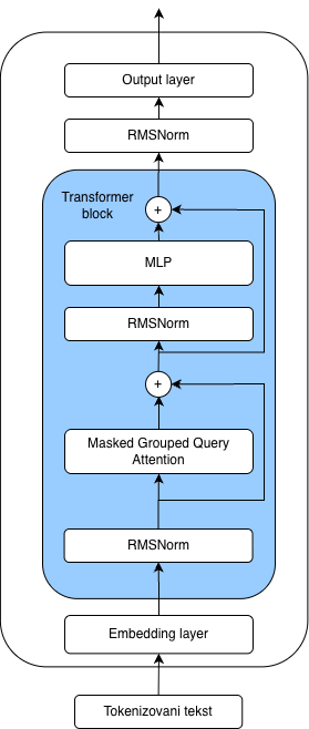
Figure 12: Llama 3 model architecture.
3.3 Qwen3
The Chinese company Alibaba has become well-known for its popular open-weight large language models under the name Qwen. Yang et al. (2025) introduced a new model in this series in May, called Qwen3. The model comes in two variants - Dense and Mixture of Experts - depending on the implementation of the multilayer perceptron within the transformer block. Dense models come in seven different sizes: 600 million, 1.7 billion, 4 billion, 8 billion, 14 billion, and 32 billion parameters. On the other hand, the Mixture of Experts models come in two sizes. The first, named 30B-A3B, has 30 billion parameters, with 3 billion parameters from the expert layer activated for each token prediction, while the second, named 235B-A22B, has a total of 235 billion parameters, with 22 billion parameters from the expert layer activated during inference.
This work will focus specifically on the Qwen3 0.6B model, which, due to its relatively small size, is suitable for use on consumer hardware. The model consists of 28 transformer blocks, making it significantly deeper compared to the LLaMA 3.2 1B model, which contains 16 transformer blocks. It should be noted that each transformer block in Qwen 3 0.6B has 16 attention heads, which is half the number present in the LLaMA 3.2 1B model. The token vector representations in the Qwen 0.6B model have 1,024 dimensions, and the maximum supported context length is 32,000 tokens. The model uses the previously mentioned grouped query attention mechanism, but for improved training stability, it also introduces QK-Norm (Dehghani et al., 2023). Yang et al. (2025) also report that the Qwen series models are trained using the Qwen tokenizer and a vocabulary of 151,669 tokens.
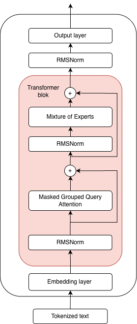
Figure 13: Qwen3 model architecture.
3.4 GPT OSS
In August of this year, Agrawal et al. (2025) released two open-source model versions under the name GPT-OSS, available in 20-billion and 120-billion parameter variants. More than six years have passed since the release of GPT-2, and we can observe differences in the architecture between that model and the new GPT-OSS models. Layer normalization has been replaced with the RMSNorm module, the multi-head self-attention mechanism has been replaced with a more efficient masked grouped-query attention mechanism, the single multilayer perceptron from the transformer block has been replaced with a mixture-of-experts module, and dropout modules have been completely omitted.
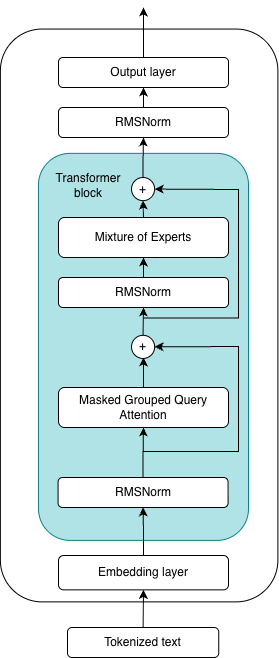
Figure 15: Architecture of the GPT OSS model
4 Implementation and analysis of components of large language models
This chapter deals with the implementation and analysis of components of large language models. All components are implemented using a deep learning framework called PyTorch (Paszke et al., 2017, 2019). The GPT-2 and Llama 3.2 model architectures were completely reimplemented for the purposes of this article. Certain components such as the singular attention head will be implemented independently of the model and are used for demonstration purposes.
4.1 High level code overview of GPT 2
                        class GPT(nn.Module):
                            """
                            GPT 2 core class
                            """
                            def __init__(self, config):
                                super().__init__()
                                self.config = config
                                # This is how HF organizes their gpt2 implementation
                                self.transformer = nn.ModuleDict(dict(
                                    wte = nn.Embedding(config.vocab_size, config.n_embd),
                                    wpe = nn.Embedding(config.block_size, config.n_embd),
                                    h = nn.ModuleList([Block(config) for _ in range(config.n_layer)]),
                                    ln_f = nn.LayerNorm(config.n_embd)
                                ))
                                self.lm_head = nn.Linear(config.n_embd, config.vocab_size, bias=False)

                                # lm_head shares the weight matrix with wte
                                # This is quite clever optimization as it turns out it helps with regularization and reduces the number of trainable parameters
                                # Additionally this does not seem correct at the first glance since wte = nn.Embedding(vocab_size, n_embd) and lm_head = nn.Linear(n_embd, vocab_size)
                                # But since lm_head is linear it will be saved as (vocab_size, n_embd) actually and that matches with dimensions of wte
                                self.transformer.wte.weight = self.lm_head.weight

                            def forward(self, idx, targets = None):
                                # idx is as tensor containg batches B of sequences T, (B, T) - T is a sequence of token ids - idx = [[14, 2435, 1234], [345, 43567, 8067]]
                                B, T = idx.size()
                                assert T <= self.config.block_size, f"Cannot forward sequence of length {T}, block size is only {self.config.block_size}"
                                # Now we create a tensor [0, 1, 2, ..., T-1] - this basically marks positions inside our sequence
                                pos = torch.arange(0, T, dtype=torch.long, device=idx.device)
                                # For each position in a sequence we will get the positional embedding
                                # Since we have T elements in the sequence we will obtain positional emedding for each element so it is a tensor (T, n_embd)
                                # Since all the batches have sequences that are of length T we pluck out the positional embedding just once
                                pos_emb = self.transformer.wpe(pos)
                                # In this step we create token embeddings for each id in a sequence for each batch - this results in (B, T, n_embd) tensor
                                tok_emb = self.transformer.wte(idx)
                                # Now we need to combine these two - since pos_e (T, n_embd) and tok_e (B, T, n_embd) PyTorch will do the broadcasting for us
                                # It basically adds a dimension B to pos_e to match the dims of tok_e
                                x = tok_emb + pos_emb

                                # Now we propagete the x which is (B, T, C) though Transformer blocks
                                for block in self.transformer.h:
                                    x = block(x)

                                # Now we do the LayerNorm one last time
                                x = self.transformer.ln_f(x)

                                # We pass x which is (B, T, n_embd) through LM head which will basically do the calssification and predict
                                # the next most probable token
                                # The output here is (B, T, vocab_size) where in the last dimension we have 50257 logits - one for each possible token in vocab
                                logits = self.lm_head(x)

                                loss = None
                                if targets is not None:
                                    loss = F.cross_entropy(logits.view(-1, logits.size(-1)), targets.view(-1))
                                return logits, loss
4.2 Implementation and analysis of different attention mechanisms
The attention mechanism is considered one of the main reasons for the success of transformers. It can essentially be viewed as a communication mechanism in which tokens exchange information with each other, and the end result is context-aware vectors. These vectors make predicting the next token a significantly easier task, because in addition to carrying information about themselves, each vector also contains information about the tokens that preceded it. This is especially true in the case of attention applied with masking for causal language modeling, where tokens in a sequence are allowed to attend only to previous tokens.
4.2.1 Single Attention Head
                        class SingleHeadAttention(nn.Module):
                            """
                            Single Head of Attention - made for demonstration purpose
                            """
                            def __init__(self, config):
                                super().__init__()
                                self.W_key = nn.Linear(config.embd_dim, config.embd_dim)
                                self.W_value = nn.Linear(config.embd_dim, config.embd_dim)
                                self.W_query = nn.Linear(config.embd_dim, config.embd_dim)


                            def forward(self, x: torch.Tensor, mask: torch.Tensor):
                                batch_size, seq_length, embd_dim = x.shape

                                # Generating Q, K and V
                                q = self.W_query(x) # (batch_size, seq_length, embd_dim)
                                k = self.W_key(x) # (batch_size, seq_length, embd_dim)
                                v = self.W_value(x) # (batch_size, seq_length, embd_dim)


                                attn_scores = (q @ k.transpose(1, 2) * (1 / (k.size(-1) ** 0.5)))


                                # Applying mask for Causal Language Modeling (self-attention)
                                attn_scores = attn_scores.masked_fill(mask, -torch.inf)


                                # Normalizing attention scores by applying row-wise softmax -> attention in each row sums up to 1
                                normalized_attn_scores = F.softmax(attn_scores, dim=-1)


                                y = normalized_attn_scores @ v


                                return y
4.2.2 Multihead Attention
Multi-Head Attention (Vaswani et al., 2017), was created as an attempt to allow the model to simultaneously consider relationships between words in a sentence from multiple perspectives. It is a way to improve the model's capacity to understand complex relationships between words in a sentence. It is implemented using separate weight matrices for keys, queries, and values for each attention head. These matrices are used to project the input and obtain the corresponding keys, queries, and values. The attention mechanism works by comparing the queries and keys, with their similarity calculated via the dot product, which is then scaled by the square root of the key vector dimension for numerical stability. The resulting query-key similarity matrix is then normalized using the softmax function. The softmax function is applied to each row of the matrix, converting it into a probability distribution, or attention distribution, which determines how much attention each token pays to the surrounding tokens. The first row of this matrix corresponds to the distributed attention of the first token, the second row corresponds to the attention of the second token, and so on. The resulting attention matrix is then multiplied by the value matrix, producing context-aware vector representations of the tokens in the input sequence for a single attention head. Before obtaining the final output of the multi-head attention operation, the outputs of all heads are concatenated and then passed through an additional linear transformation using the matrix Wo. This transformation serves to integrate the information obtained from each individual attention head.
Since this module is computationally very expensive, with a time complexity of O(n^2 d), which, given that d is a constant independent of input length, can be viewed as O(n^2), and contains a large number of parameters, it remains a frequent subject of research aimed at finding equally effective but less demanding variants. The quadratic complexity of the attention mechanism is also the main reason for the practical limitations on the context length of these models.
                        class CausalSelfAttention(nn.Module):
                            """
                            Multiheaded Causal Self Attention
                            """
                            def __init__(self, config):
                                super().__init__()
                                assert config.n_embd % config.n_head == 0
                                # Key, query, value projections for all heads but in a batch
                                self.c_attn = nn.Linear(config.n_embd, 3 * config.n_embd)
                                # output projection
                                self.c_proj = nn.Linear(config.n_embd, config.n_embd)
                                self.n_head = config.n_head
                                self.n_embd = config.n_embd
                                # mask - called bias by OpenAI/HF
                                self.register_buffer("bias", torch.tril(torch.ones(config.block_size, config.block_size)).view(1, 1, config.block_size, config.block_size))


                            def forward(self, x: torch.Tensor):
                                B, T, C = x.size() # Batch size, sequence length, embedding dimensionality (token embedding length)


                                # We will first calculate query, key and values for ALL HEADS
                                # nh is "number of heads", hs is "head size", and C (num of channels) = nh * ns
                                # e.g in GPT-2 (124M), n_heads = 12, hs = 64, so nh * ns = C = 768 channels in Transformer
                                # each head outputs sequence of vectors of a size 64, so in multiheaded self attention the last step is to concatenate outputs from all the heads
                                # by doing this concatenation we effectively restore the dimensions of original embeddings and preserve
                                # different information we obtained from each head

                                # Joined Q, K, V values for all the heads
                                # attention(Q,K,V) = softmax((Q @ K^T) * 1/sqrt(n_embed)) @ V
                                # For a single head -> x @ Wq = Q, x @ Wk = 0, x @ Wv = V
                                # In multiheaded attention Wq holds weights for all the heads, same goes for Wk, Wv
                                # So q, k, v here are q for all the heads, k for all the heads, v for all the heads
                                # Since x is (B, T, C) and it passes through linear layer with weight matrix of (C, 3 * C)
                                # qkv is (B, T, 3 * C)
                                qkv = self.c_attn(x)


                                # Each of them will be of the size (B, T, C)
                                q, k, v = qkv.split(self.n_embd, dim=2)

                                # Now we want to retain the notion of separate q, k, v per head
                                # using .view() we transform (B, T, C) into (B, T, nh, n_embed / n_heads)
                                # We transpose (B, T, nh, hs) into (B, nh, T, hs) so this is the tensor that holds Q
                                # It hold data for B batches, each batch has 12 heads, each sequence is of length T, and each query is of hs length
                                q = q.view(B, T, self.n_head, C // self.n_head).transpose(1, 2)
                                # We repeat for all the others
                                k = k.view(B, T, self.n_head, C // self.n_head).transpose(1, 2)
                                v = v.view(B, T, self.n_head, C // self.n_head).transpose(1, 2)


                                # We calculate the attention - we transpose only the last two dims of k
                                # (B, nh, T, hs) @ (B, nh, hs, T) = (B, nh, T, T)
                                att = (q @ k.transpose(-2, -1)) * (1.0 / math.sqrt(k.size(-1)))

                                # For every batch, and for every head in a batch, we will look at all T sequences of length T
                                # Since bias is tensor (1, 1, bs, bs) where (bs, bs) is a lower triangular matrix
                                # We will overlay it over each (T, T) matrix in (B, nh, T, T) tensor and turn all the 0 to -inf
                                # This will essentially mask the future tokens so the earlyer ones can't attend to them
                                # We use -inf and not 0 because this will have benefits for softmax
                                # This is also called autoregressive mask
                                att = att.masked_fill(self.bias[:, :, :T, :T] == 0, float('-inf'))

                                # Now we apply softmax along each row in each sequence T
                                # So if we look at row i in TxT matrix and pluck it out
                                # We will see how much attention token at position i gives to all the other tokens is sequence T
                                # So once we apply softmax on a row basis we normalized attention that each token i pays attention to all the other tokens in the sequence and it sums to 1
                                att = F.softmax(att, dim=-1)

                                # Now we need to do att @ V so we obtain modified values of embeddings based on the attention
                                # (B, nh, T, T) @ (B, nh, T, hs) = (B, nh, T, hs)
                                y = att @ v


                                # Alternatively previous 4 lines could have been commented out and we could use flash attention
                                # y = F.scaled_dot_product_attention(q, k, v, is_causal=True)


                                # Now we first transpose this tensor so we get (B, T, nh, hs)
                                # We then need to use contiguous() function to allocate continuous block of memory for our tensor
                                # This will ensure us that tensor's data is stored in memory in sequential, row-major order.
                                # Now we can perform reshaping of our tensor, where we concatenate outputs of each head
                                y = y.transpose(1, 2).contiguous().view(B, T, C)


                                # Finally we just project the output through the linear layer
                                y = self.c_proj(y)
                                return y
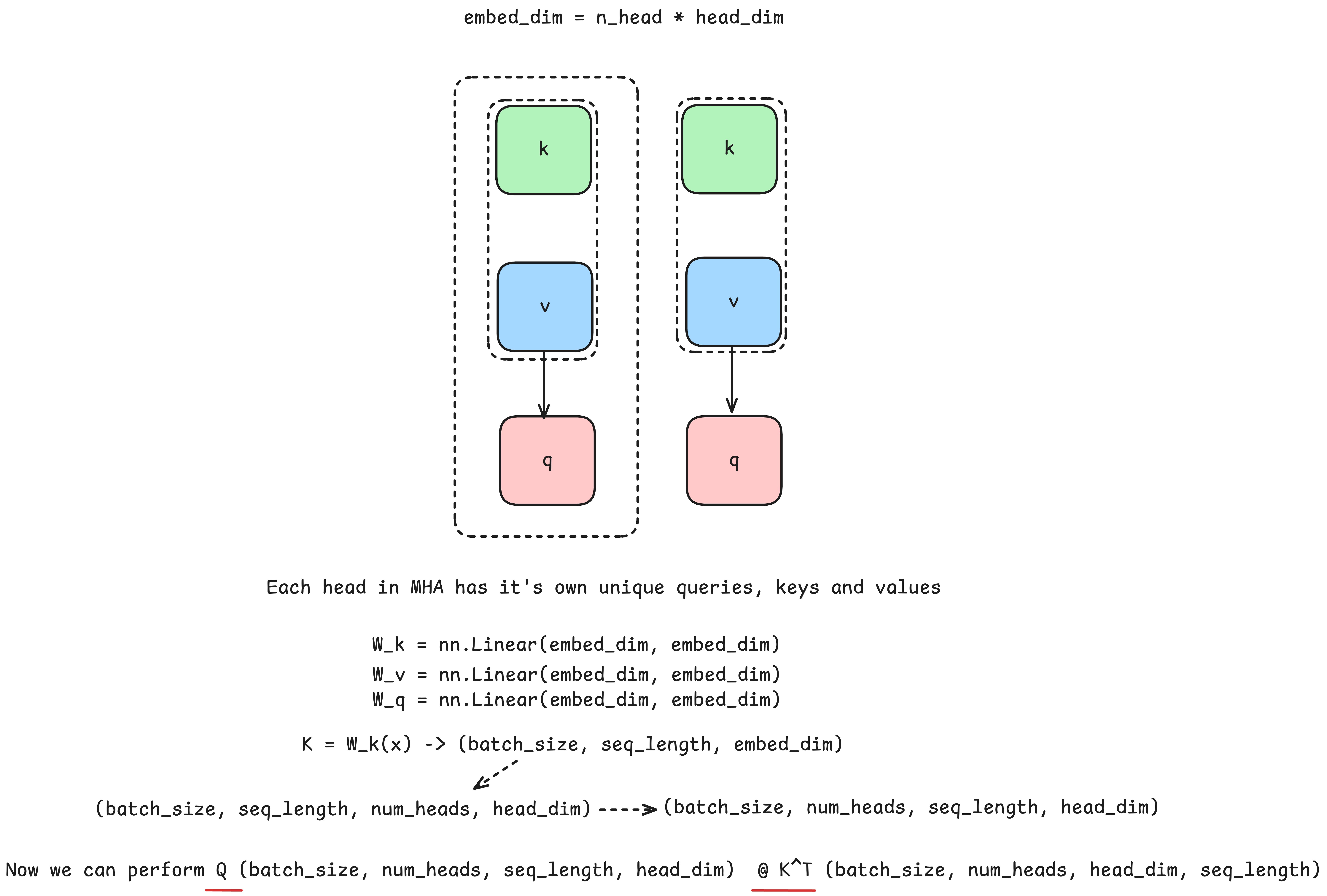
Figure 15: Multihead Attention
4.2.3 Grouped Query Attention
Grouped Query Attention has the goal of reducing the number of parameters used in the attention module. The main idea of this attention variant is that, instead of every head having its own keys and values for each query, multiple attention heads share the same keys and values. With a bit of additional tensor manipulation, the rest of the implementation is nearly identical to traditional multi-head attention. The code shown in this section corresponds to the attention module used in the LLaMA 3.2 model.
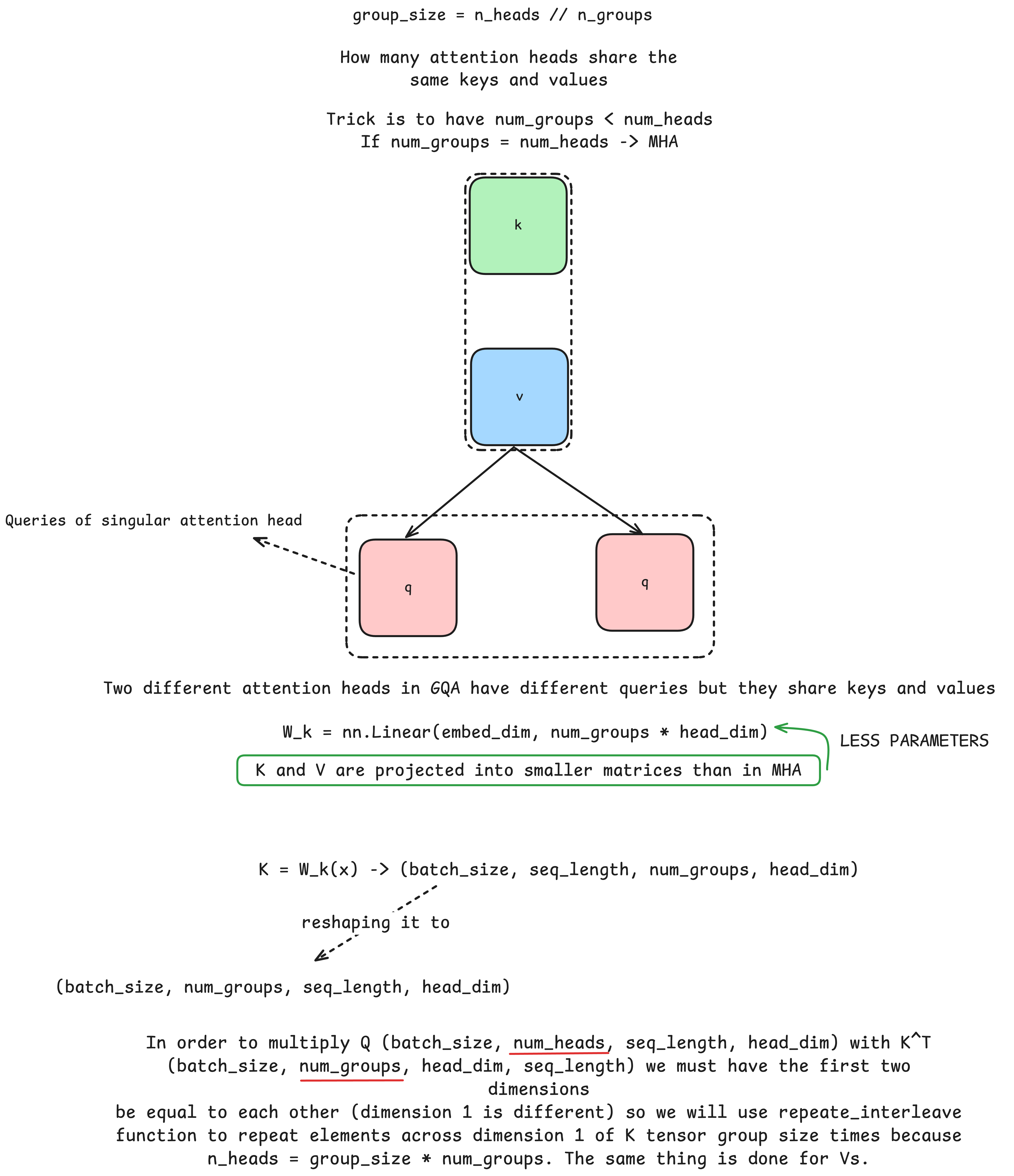
Figure 16: Groped Query Attention
                        class GroupedQueryAttention(nn.Module):
                            """
                            This class represents implementation of Grouped Query Attention Mechanism found in Llama 3.2 model
                            GQA reduces the number of parameters needed by sharing Keys and Values between attention heads
                            """
                            def __init__(self, config: LlamaConfig):
                                super().__init__()
                                self.d_out = config.emb_dim
                                self.num_heads = config.n_heads
                                self.head_dim = config.emb_dim // config.n_heads
                                self.num_kv_groups = config.n_kv_groups
                                self.group_size = config.n_heads // config.n_kv_groups
                                self.W_key = nn.Linear(config.emb_dim, self.num_kv_groups * self.head_dim, bias=False, dtype=config.dtype) # add dtypes
                                self.W_value = nn.Linear(config.emb_dim, self.num_kv_groups * self.head_dim, bias=False, dtype=config.dtype)
                                self.W_query = nn.Linear(config.emb_dim, self.d_out, bias=False, dtype=config.dtype)
                                self.out_proj = nn.Linear(self.d_out, self.d_out, bias=False, dtype=config.dtype)
                                # kv_cache
                                self.register_buffer("cache_k", None, persistent=False)
                                self.register_buffer("cache_v", None, persistent=False)


                            def forward(self,x: torch.Tensor,
                                        sin: torch.Tensor,cos: torch.Tensor,
                                        mask: torch.Tensor, use_cache: bool = False, start_pos = 0):
                                batch_size, seq_length, d_in = x.shape

                                # Generating Q, K and V
                                q = self.W_query(x) # (batch_size, seq_length, d_out)
                                k = self.W_key(x) # (batch_size, seq_length, self.num_kv_groups * self.head_dim)
                                v = self.W_value(x) # (batch_size, seq_length, self.num_kv_groups * self.head_dim)


                                # Reshaping
                                q = q.view(batch_size, seq_length, self.num_heads, self.head_dim)
                                k = k.view(batch_size, seq_length, self.num_kv_groups, self.head_dim)
                                v = v.view(batch_size, seq_length, self.num_kv_groups, self.head_dim)


                                q = q.transpose(1, 2) # (batch_size, num_heads, seq_length, head_dim)
                                k = k.transpose(1, 2) # (batch_size, num_kv_groups, seq_length, head_dim)
                                v = v.transpose(1, 2) # (batch, num_kv_groups, seq_length, head_dim)


                                # RoPE Application -> Rotating queries and keys
                                if cos is not None:
                                    q = _apply_rope(q, cos, sin, start_pos)
                                    k = _apply_rope(k, cos, sin, start_pos)


                                if use_cache:
                                    if self.cache_k is None:
                                        self.cache_k = k
                                        self.cache_v = v
                                    else:
                                        # x shape (batch_size, 1, embd_dim)
                                        # q shape (batch_size, 1, d_out)
                                        # q after reshaping (batch_size, num_heads, seq_length, head_dim)
                                        # k and v shape (batch_size, seq_len, self.num_kv_groups * self.head_dim)
                                        # k and v after reshaping (batch_size, seq_len, num_kv_groups, head_dim) after reshaping
                                        self.cache_k = torch.cat((self.cache_k, k), dim=2)
                                        self.cache_v = torch.cat((self.cache_v, v), dim=2)

                                        # Now we take all the values from cache so we can get complete K and V matrices for
                                        k = self.cache_k
                                        v = self.cache_v


                                k = k.repeat_interleave(self.group_size, dim=1) # (batch_size, num_kv_groups * group_size = num_heads, seq_length, head_dim)
                                v = v.repeat_interleave(self.group_size, dim=1) # (batch_size, num_heads, seq_length, head_dim)

                                attn_scores = (q @ k.transpose(2, 3) * (1 / (k.size(-1) ** 0.5))) # (QK^T)/sqrt(dim_k)

                                # Applying mask for Causal Language Modeling
                                attn_scores.masked_fill(mask, -torch.inf)

                                # Normalizing attention scores by applying row-wise softmax -> attention in each row sums up to 1
                                normalized_attn_scores = F.softmax(attn_scores, dim=-1)


                                # (batch_size, num_heads, seq_length, seq_length) x (batch_size, num_heads, seq_length, head_dim) = (batch_size, num_heads, seq_length, head_dim)
                                y = normalized_attn_scores @ v
                                # Transposing (batch_size, num_heads, seq_length, head_dim) to (batch_size, seq_length, num_heads, head_dim)
                                # Reshaping output tensor (batch_size, seq_length, num_heads, head_dim) so we get (batch_size, seq_length, d_in)
                                y = y.transpose(1, 2).contiguous().view(batch_size, seq_length, d_in)

                                y = self.out_proj(y)

                                return y

                            def reset_kv_cache(self):
                                self.cache_k = None
                                self.cache_v = None
4.2.4 Sliding window attention
Sliding window attention is a mechanism introduced in a paper published by Beltagy et al. (2020). The goal of this work was to improve the operation of the transformer on longer sequences and create a more efficient attention mechanism. The authors reduce the quadratic time and memory complexity of the standard attention module by introducing a sliding-window mechanism in which each current token does not attend to the entire preceding context but only to w tokens that precede it. In this way, they create an algorithm whose time and memory complexity is linear, that is, O(nw) where n is the length of the sequence, and w is the length of the context to which attention will be paid. Modern architectures of large language models today very often combine quadratic complexity attention layers with layers that implement a sliding window of attention achieving good results with certain time and memory savings realized by this implementation.
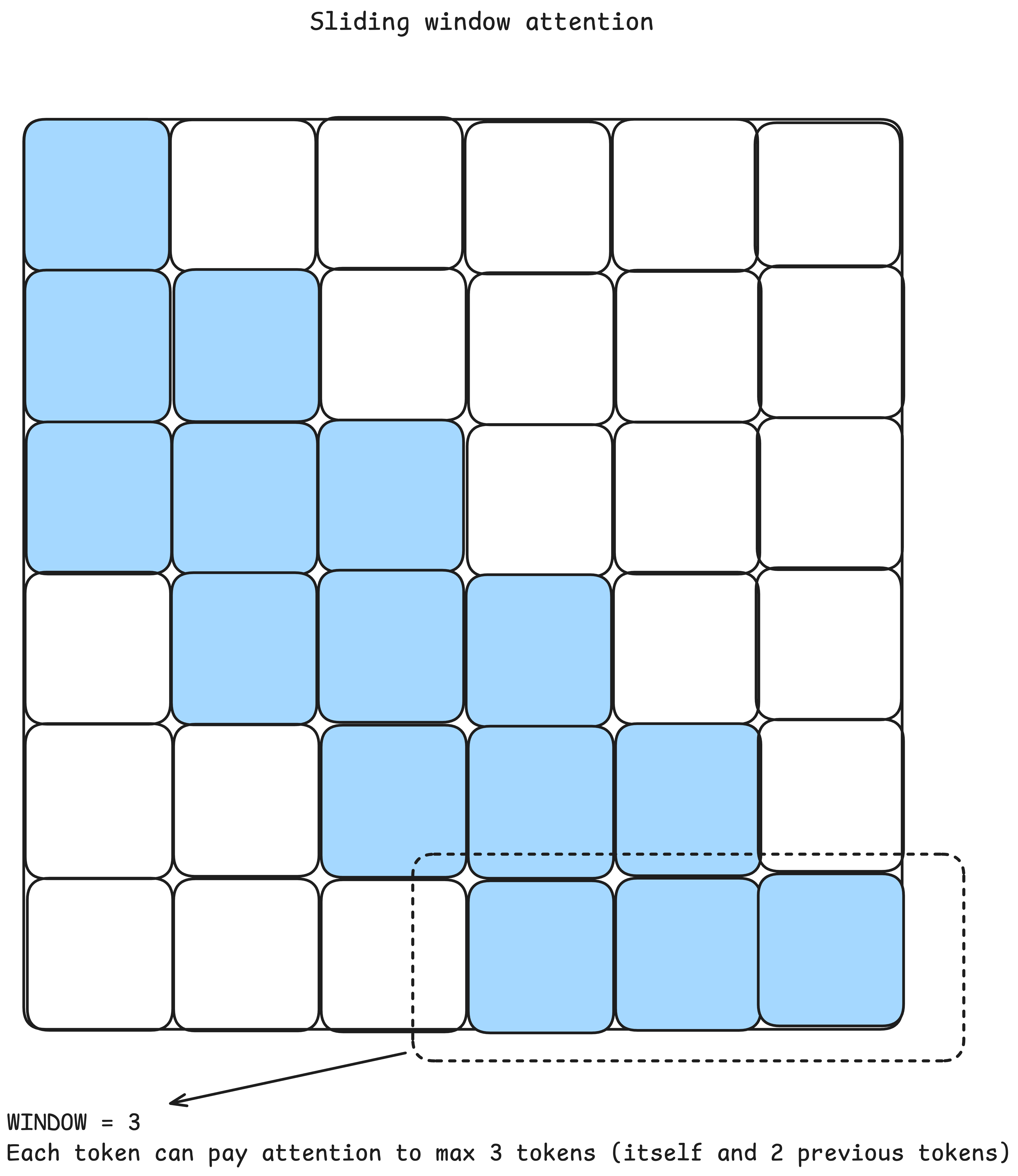
Figure 17: Sliding window attention pattern. Again, summed values of attention weights (blue) in every single row will be equal to 1 (after applying softmax which will convert raw dot product values between keys and queries into a probability distribution) while the transparent squares get assigned value of 0.
4.3 Implementation and analysis of different normalization techniques
One of the techniques important for the success of deep neural networks is sporadic normalization between layers, which has been shown to contribute to more stable training by reducing the problem of exploding or vanishing gradients. Normalization leads to a faster convergence and enables more stable training of deep neural networks. The usual procedure is to normalize the values after applying the activation function, but it is possible to normalize the gradients as well as the weights.
RMSNorm is a computationally more efficient way of normalization compared to layer normalization, which is also found in large language models. It does not require the calculation of the mean and standard deviation, but rather the input is scaled by the root mean square sum of the input values which are then multiplied by the parameters adjusted through training. It should be noted that a small epsilon value is added under the root itself to avoid potential division by zero.
Another noticeable difference between the original transformer and newer language models is the placement of the normalization layers. In most newer models, it is now located immediately before the attention module, which was not the case with the original transformer, which performed normalization after the attention module.
4.3.1 Layer Norm
                        class LayerNorm(nn.Module):
                            """
                            This class represents implementation of Layer norm.
                            PyTorch offers Layer norm but I will implement it from scratch for educational purposes
                            More can be found here: https://docs.pytorch.org/docs/stable/generated/torch.nn.LayerNorm.html
                            """
                            def __init__(self, embd_dim: int, epsilon: float = 1e-5):
                                super().__init__()
                                self.epsilon = epsilon
                                self.embd_dim = embd_dim
                                self.scale_weight = nn.Parameter(torch.ones(embd_dim)).float()
                                self.shift_weight = nn.Parameter(torch.zeros(embd_dim)).float()


                            def forward(self, x: torch.Tensor):
                                mean = x.mean(dim=-1, keepdim=True)
                                var = x.var(dim=-1, unbiased=False ,keepdim=True)
                                x_normalized = (x - mean) / torch.sqrt(var + self.epsilon)
                                x_normalized = x_normalized * self.scale_weight + self.shift_weight
                                return x_normalized.to(dtype=x.dtype)
4.3.2 RMSNorm
                        class RMSNormLayer(nn.Module):
                            """
                            This class represents the implementation of the RMSNorm layer.
                            PyTorch offers layer RMSNorm layer but I will implement it from scratch for educational purposes
                            More can be found here: https://docs.pytorch.org/docs/stable/generated/torch.nn.RMSNorm.html
                            """
                            def __init__(self, embd_dim: int, epsilon: float = 1e-5):
                                super().__init__()
                                self.epsilon = epsilon
                                self.embd_dim = embd_dim
                                self.weight = nn.Parameter(torch.ones(embd_dim)).float()


                            def forward(self, x: torch.Tensor):
                                root_mean_squares = torch.sqrt(x.pow(2).mean(dim=-1, keepdim=True) + self.epsilon)
                                x_normalized = x / root_mean_squares
                                return (x_normalized * self.weight).to(dtype=x.dtype)
4.4 Implementation and analysis of different position encoding mechanisms
Transformer creates context-aware vector representations through its attention mechanism, and in order to achieve this effectively, it is necessary to pass its position to the attention module with each token. Without information about the position, the transformer would not be able to distinguish the same words or tokens, which are located in different positions in the sequence, and would produce equal vector representations for them, which is not desirable. Let's look at the sentence "The dog chased the dog" and notice that the first dog is the subject that performs an action on the second dog, which is the object in this sentence. Without information about the order in the sequence or the position of each token, the vector representation of this sequence would contain two identical vectors referring to the same word, and the model would not be able to recognize the difference between the subject and the object in this sentence. In order to avoid situations similar to the one mentioned above, layers responsible for entering, or encoding, information about the position of each token are introduced into the transformer architecture.
4.4.1 Encoding information using sinusoidal functions
The original transformer introduced sinusoidal embeddings and relies on a table of values that is calculated using information about the position of the tokens in the sequence, the vector component indices, and the sinusoidal functions. The basic idea is that the lower indices of the components of the semantic vectors correspond to high-frequency sinusoidal waves capable of capturing small changes in context, while the higher indices correspond to lower-frequency waves that retain information that is unique. It is important to note that in this way the number of model parameters is reduced because this way of encoding does not require the model to learn the table during training, but it can be calculated based on the characteristics of the architecture. After creating a table containing information related to each possible position in the sequence, the authors of the original transformer decided to add, based on the position in the sequence, to the semantic embedding of tokens obtained from the embedding layer, the corresponding vector found in the table of sine function values that we previously calculated. In this way, successful propagation of token position data through further layers of the model is ensured.
                        def sinusoidal_positional_encoding(max_position, d_model):
                            """
                            Table of sinusoidal position embeddings
                            """
                            position = torch.arange(max_position).unsqueeze(1)
                            div_term = 1 / (10000 ** (torch.arange(0, d_model, 2) / d_model))
                            pe = torch.zeros((max_position, d_model))
                            pe[:, 0::2] = torch.sin(position * div_term)
                            pe[:, 1::2] = torch.cos(position * div_term)

                            return pe
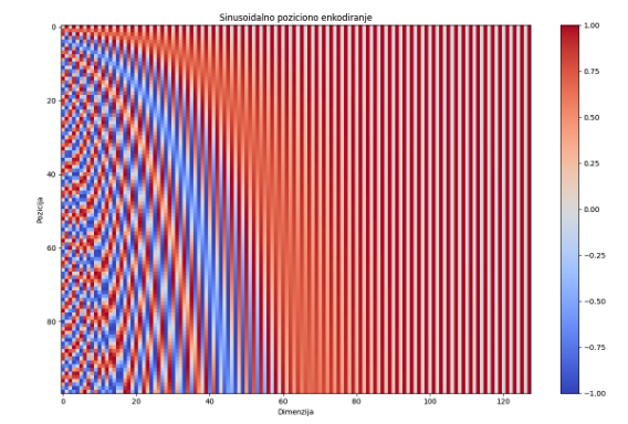
Figure 18: Sinusoidal embedding table - Rows represent position of a token in a sequence while columns represent dimension of an embedding vector
4.4.2 Incorporating Positional Information via trainable parameters
Another way to inject positional information is by using parameters learned during training. By using a linear layer of appropriate dimensions, it is possible to obtain a matrix containing vectors that carry positional information. By adding the appropriate position vector to the semantic vector, efficient association of positional information is achieved, which is further propagated through the model. This type of positional encoding is used in the GPT-2 model.
4.4.3 RoPE
Llama uses an approach called RoPE (Rotary Positional Encoding) presented in a paper called RoFormer (Su et al., 2021). The main idea of this work was that instead of adding information to the semantic vector, it is actually rotated. In this way, the original semantic vector, i.e. its magnitude is completely preserved, and its components are rotated depending on the position and index in the vector. Essentially this work is an extension of sinusoidal embeddings, but instead of adding a newly calculated vector, we use sinusoidal functions, positions and indices to calculate the corresponding element of the rotation matrix. Each of the embeddings is primarily divided into pairs of its components, to which the rotation matrix in is then applied R2. Smaller indices will be rotated faster relative to the bigger indices so the idea from sinusoidal embeddings is retained (smaller indeces oscillate faster while the bigger ones oscillate slower). Since pairs of coordinates from a vector can be viewed as complex numbers, and rotation as multiplication by a complex number, different ways of implementing this module can be encountered. In particular, I first stuck to the implementation proposed in the original paper where I used pairs of adjacent vector components, however this did not give good results because Llama was actually trained to split the original input vector into two equal halves and then match the elements at the same indices within those two newly created vectors. Also, it should be noted that this rotation is actually applied within the attention module to queries and keys before the actual calculation of attention.
Another one of the modifications present in the concrete implementation is frequency scaling. A paper called YaRN (Peng et al., 2023) aimed to make RoPE work better with sequences that are longer than those on which the model was originally trained. In the specific implementation of Llama, this is achieved by dividing it into three wavelength zones: short, medium and long, to which appropriate scaling is applied. The problem arises with long sequences because periodicity occurs in waves that correspond to big indices, that is, waves of long wavelength, which should contain unique information. The appearance of periodicity at such places could confuse the model and hurt performance, so YaRN proposes scaling these wavelengths, effectively extending their period. In this way, these waves become aperiodic for the model, and the uniqueness of their values in a certain interval is preserved. Small wavelengths remain unchanged, while mid-range wavelengths are scaled to provide a smooth transition from low to high wavelengths.
                        def _precompute_rope_params(head_dim, config:LlamaConfig):
                            # integer -> binary -> sinusoidal -> RoPE
                            # RoPE does not pollute the semantics of token embeddings because we do not add vector containing the positional info, we rotate queries and keys
                            # Encodes both absolute and relative position information
                            # theta = position * omega
                            # omega = 1 / 500000 ^ (2i/dim)
                            # rot matrix = [[cos(theta) -sin(theta)] [sin(theta) cos(theta)]]
                            # Token embedding gets split into groups of 2 so there are dim // 2 groups of 2 that get rotated
                            # Lower indices in token embeddings oscillate more quickly capturing small changes
                            assert head_dim % 2 == 0, "Head dimension must be divisible by 2"
                            position = torch.arange(0, config.context_length, dtype=torch.float32).view(config.context_length, 1) # converting tensor of rank 1 to -> (context_length, 1)
                            i = torch.arange(0, head_dim, 2, dtype=torch.float32) # (head_dim/2,) -> Number of groups (pairs of 2) in attention head [x0, x1, x2, x3] -> (x0, x1), (x2, x3)
                            omega = 1.0 / torch.pow(config.rope_base, (i / head_dim))
                            # Scaling frequencies - YaRN paper - this helps with long sequences
                            if config.rope_freq is not None:
                                low_freq_wavelen = config.rope_freq.original_context_length / config.rope_freq.low_freq_factor
                                high_freq_wavelen = config.rope_freq.original_context_length / config.rope_freq.high_freq_factor


                                wavelen = 2 * torch.pi / omega #

                                inv_freq_llama = torch.where(
                                    wavelen > low_freq_wavelen, omega / config.rope_freq.factor, omega
                                )


                                smooth_factor = (
                                    config.rope_freq.original_context_length / wavelen
                                    - config.rope_freq.low_freq_factor
                                ) / (
                                    config.rope_freq.high_freq_factor - config.rope_freq.low_freq_factor
                                )


                                smoothed_inv_freq = (
                                    (1 - smooth_factor) * (omega / config.rope_freq.factor)
                                    + smooth_factor * omega
                                )


                                is_medium_freq  = (wavelen <= low_freq_wavelen) & (wavelen > high_freq_wavelen)
                                inv_freq_llama = torch.where(is_medium_freq, smoothed_inv_freq, inv_freq_llama)
                                omega = inv_freq_llama

                            omega = omega.view(1, int(head_dim/2)) # (1, head_dim/2)
                            theta = position * omega # (context_length, head_dim/2) -> matrix that contains angle for each position and group
                            theta = torch.cat((theta, theta), dim=1) # (context_length, head_dim) -> matrix that contains angle for each position and index in attention head
                            cos = torch.cos(theta)
                            sin = torch.sin(theta)

                            return cos, sin


                        # This will be used inside my GQA to rotate queries and keys
                        def _apply_rope(x: torch.Tensor, cos: torch.Tensor, sin: torch.Tensor, start_pos: int=0):
                            batch_size, num_heads, seq_len, head_dim = x.shape
                            assert head_dim % 2 == 0, "Head dimension must be divisible by 2"
                            # Split x into two even parts on head_dim
                            x_first_half = x[..., : head_dim // 2]
                            x_second_half = x[..., head_dim // 2 :]
                            cos = cos[start_pos:start_pos+seq_len, :].reshape((1, 1, seq_len, -1))
                            sin = sin[start_pos:start_pos+seq_len, :].reshape((1, 1, seq_len, -1))
                            # o1' = cos * x_first_half - x_second_half * sin
                            # o2' = sin * x_first_half + x_second_half * cos
                            rotated = torch.cat((-x_second_half, x_first_half), dim=-1)
                            x_rotated = (x * cos) + (rotated * sin)

                            return x_rotated.to(dtype=x.dtype)
4.5 Implementation and analysis of MLPs present in large language models
The total number of parameters of the smallest model from the GPT-2 series is 124,439,808. If we look at the transformer block, more precisely the multilayer perceptron within this block, we can see that it has 4,722,432 parameters. The smallest model from the GPT-2 series has 12 sequential transformer blocks, and the number of parameters of multilayer perceptrons from transformer blocks actually amounts to 56,669,184, which is about 45% of the total number of parameters of the entire model.
The Llama 3.2 1B model has a total of 1,498,482,688 parameters, while the total number of parameters in the multilayer perceptrons in the 16 transformer blocks of this model is 805,306,368, which represents about 54% of the total number of parameters.
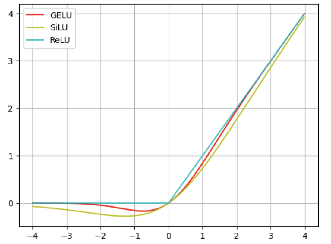
Figure 19: Different activation functions used in LLMs
4.5.1 Mixture of Experts
The Mixture of Experts module was not invented by DeepSeek, but they are the ones who made it popular. The MoE module replaces the traditional MLP found in a transformer block and introduces experts instead. Each expert is an MLP, so MoE essentially replaces one large MLP module with a collection of smaller MLP modules that specialize during training. As we have seen above, the MLP appears in every transformer block and accounts for a large portion of a large language model's parameters, so replacing a single large module with a group of smaller ones actually increases the model's total parameter count. However, the main advantage of this approach is that only a small subset of experts is activated when processing each token, meaning that using an MoE layer gives the model additional parameters to store knowledge without sacrificing speed or performance during inference. A good example of a model that uses this approach is DeepSeek-V3, which has 256 experts per MoE module and a total of 671 billion parameters.
4.5.2 Output projection layer
This is the MLP that is used to project tokens from the final hidden states of the decoder block to vocabulary space. Outputs of the MLP are called logits (unnormalized log-probabilities) and we produce one for every token i in the vocabulary V. We use these logits to obtain probability distribution over the vocabulary by applying the softmax function on them. There are different decoding strategies, meaning there are different ways to choose the next token, but one possible way would be to pick the token with the highest probability as the model's prediction for the next word (or sub-word). This is called Greedy Decoding. In many models, the weight matrix W of the output projection layer is tied to the weight matrix of the initial input embedding layer. This is called weight tying and it allows us to reduce the number of trainable parameters in our model without damaging the performance.
Outro
Congratulations! You have made it to the very end of this post. I hope that you've enjoyed reading it and that you've learned something new. This was my first blog ever so I would appreciate feedback from you guys. In the following chapters I plan to cover Training of LLMs [Part 2] after which I will focus on Inference [Part 3] and Optimizations [Part 4].
5 Resources
- Agarwal, S., Ahmad, L., Ai, J., Altman, S., Applebaum, A., Arbus, E., Arora, R. K., Bai, Y., Baker, B., Bao, H., Barak, B., Bennett, A., Bertao, T., Brett, N., Brevdo, E., Brockman, G., Bubeck, S., Chang, C., Chen, K., . . . Zhao, S. (2025). gpt-oss-120b & gpt-oss-20b Model Card. arXiv.org. https://doi.org/10.48550/arXiv.2508.10925
- Ba, J. L., Kiros, J. R., & Hinton, G. E. (2016). Layer normalization. arXiv (Cornell University). https://doi.org/10.48550/arxiv.1607.06450
- Bahdanau, D., Cho, K., & Bengio, Y. (2014). Neural machine translation by jointly learning to align and translate. arXiv (Cornell University). https://doi.org/10.48550/arxiv.1409.0473
- Bengio, Y., Ducharme, R., Vincent, P., & Janvin, C. (2003). A neural probabilistic language model. Journal of Machine Learning Research, 3, 1137-1155.
- Beltagy, I., Peters, M. E., & Cohan, A. (2020). Longformer: The Long-Document Transformer. arXiv (Cornell University). https://doi.org/10.48550/arxiv.2004.05150
- Brown, T. B., Mann, B., Ryder, N., Subbiah, M., Kaplan, J., Dhariwal, P., Neelakantan, A., Shyam, P., Sastry, G., Askell, A., Agarwal, S., Herbert-Voss, A., Krueger, G., Henighan, T., Child, R., Ramesh, A., Ziegler, D. M., Wu, J., Winter, C., . . . Amodei, D. (2020). Language Models are Few-Shot Learners. arXiv (Cornell University). https://doi.org/10.48550/arxiv.2005.14165
- Dao, T., Fu, D. Y., Ermon, S., Rudra, A., & Ré, C. (2022). FlashAttention: Fast and Memory-Efficient Exact Attention with IO-Awareness. arXiv (Cornell University). https://doi.org/10.48550/arxiv.2205.14135
- Dehghani, M., Djolonga, J., Mustafa, B., Padlewski, P., Heek, J., Gilmer, J., Steiner, A., Caron, M., Geirhos, R., Alabdulmohsin, I., Jenatton, R., Beyer, L., Tschannen, M., Arnab, A., Wang, X., Riquelme, C., Minderer, M., Puigcerver, J., Evci, U., . . . Houlsby, N. (2023). Scaling vision transformers to 22 billion parameters. arXiv (Cornell University). https://doi.org/10.48550/arxiv.2302.05442
- DeepSeek-Ai, Guo, D., Yang, D., Zhang, H., Song, J., Zhang, R., Xu, R., Zhu, Q., Ma, S., Wang, P., Bi, X., Zhang, X., Yu, X., Wu, Y., Wu, Z. F., Gou, Z., Shao, Z., Li, Z., Gao, Z., . . . Zhang, Z. (2025). DeepSeek-R1: Incentivizing reasoning capability in LLMs via Reinforcement Learning. arXiv (Cornell University). https://doi.org/10.48550/arxiv.2501.12948
- Devlin, J., Chang, M., Lee, K., & Toutanova, K. (2018). BERT: Pre-training of Deep Bidirectional Transformers for Language Understanding. arXiv (Cornell University). https://doi.org/10.48550/arxiv.1810.04805
- Grattafiori, A., Dubey, A., Jauhri, A., Pandey, A., Kadian, A., Al-Dahle, A., Letman, A., Mathur, A., Schelten, A., Vaughan, A., Yang, A., Fan, A., Goyal, A., Hartshorn, A., Yang, A., Mitra, A., Sravankumar, A., Korenev, A., Hinsvark, A., . . . Ma, Z. (2024). The Llama 3 Herd of Models. arXiv.org. https://doi.org/10.48550/arXiv.2407.21783
- He, K., Zhang, X., Ren, S., & Sun, J. (2015). Deep Residual Learning for Image Recognition. arXiv (Cornell University). https://doi.org/10.48550/arxiv.1512.03385
- Hu, E. J., Shen, Y., Wallis, P., Allen-Zhu, Z., Li, Y., Wang, S., Wang, L., & Chen, W. (2021, October 16). Lora: Low-rank adaptation of large language models. arXiv.org. https://arxiv.org/abs/2106.09685
- Kwon, W., Li, Z., Zhuang, S., Sheng, Y., Zheng, L., Yu, C. H., Gonzalez, J. E., Zhang, H., & Stoica, I. (2023). Efficient Memory Management for Large Language Model Serving with PagedAttention. arXiv (Cornell University). https://doi.org/10.48550/arxiv.2309.06180
- Mikolov, T., Chen, K., Corrado, G. S., & Dean, J. (2013). Efficient estimation of word representations in vector space. arXiv (Cornell University). https://doi.org/10.48550/arxiv.1301.3781
- Mikolov, T., Karafiát, M., Burget, L., Černocký, J., & Khudanpur, S. (2010). Recurrent neural network based language model. Interspeech 2022. https://doi.org/10.21437/interspeech.2010-343
- Meta's LLaMa license is not Open Source. (2023, July 20). Open Source Initiative. https://opensource.org/blog/metas-llama-2-license-is-not-open-source
- Meta's LLaMa license is still not Open Source. (2025, February 18). Open Source Initiative. https://opensource.org/blog/metas-llama-license-is-still-not-open-source
- Peters, M. E., Neumann, M., Iyyer, M., Gardner, M., Clark, C., Lee, K., & Zettlemoyer, L. (2018). Deep contextualized word representations. arXiv (Cornell University). https://doi.org/10.48550/arxiv.1802.05365
- Radford, A., Narasimhan, K., Salimans, T., & Sutskever, I. (2018). Improving language understanding by generative pre-training. OpenAI. https://cdn.openai.com/research-covers/language-unsupervised/language_understanding_paper.pdf
- Radford, A., Wu, J., Child, R., Luan, D., Amodei, D., & Sutskever, I. (2019). Language models are unsupervised multitask learners. OpenAI. https://cdn.openai.com/better-language-models/language_models_are_unsupervised_multitask_learners.pdf
- Paszke, A., Gross, S., Chintala, S., Chanan, G., Yang, E., DeVito, Z., Lin, Z., Desmaison, A., Antiga, L., & Lerer, A. (2017). Automatic differentiation in PyTorch. OpenReview. https://openreview.net/forum?id=BJJsrmfCZ
- Paszke, A., Gross, S., Massa, F., Lerer, A., Bradbury, J., Chanan, G., Killeen, T., Lin, Z., Gimelshein, N., Antiga, L., Desmaison, A., Köpf, A., Yang, E., DeVito, Z., Raison, M., Tejani, A., Chilamkurthy, S., Steiner, B., Fang, L., . . . Chintala, S. (2019). PyTorch: An Imperative Style, High-Performance Deep Learning Library. arXiv (Cornell University). https://doi.org/10.48550/arxiv.1912.01703
- Peng, B., Quesnelle, J., Fan, H., & Shippole, E. (2023b). YARN: Efficient context window extension of large language models. arXiv (Cornell University). https://doi.org/10.48550/arxiv.2309.00071
- Raschka, S. (2024). Build a large language model (From scratch). Simon and Schuster.
- Rosenfeld, R. (2000). Two decades of statistical language modeling: Where do we go from here? Proceedings of the IEEE, 88(8), 1270–1278.
- Sennrich, R., Haddow, B., & Birch, A. (2015). Neural Machine Translation of Rare Words with Subword Units. arXiv (Cornell University). https://doi.org/10.48550/arxiv.1508.07909
- Su, J., Lu, Y., Pan, S., Murtadha, A., Wen, B., & Liu, Y. (2021, April 20). RoFormer: Enhanced Transformer with Rotary Position Embedding. arXiv.org. https://arxiv.org/abs/2104.09864
- Touvron, H., Lavril, T., Izacard, G., Martinet, X., Lachaux, M., Lacroix, T., Rozière, B., Goyal, N., Hambro, E., Azhar, F., Rodriguez, A., Joulin, A., Grave, E., & Lample, G. (2023). LLAMA: Open and Efficient Foundation Language Models. arXiv (Cornell University). https://doi.org/10.48550/arxiv.2302.13971
- Touvron, H., Martin, L., Stone, K., Albert, P., Almahairi, A., Babaei, Y., Bashlykov, N., Batra, S., Bhargava, P., Bhosale, S., Bikel, D., Blecher, L., Ferrer, C. C., Chen, M., Cucurull, G., Esiobu, D., Fernandes, J., Fu, J., Fu, W., . . . Scialom, T. (2023). Llama 2: Open foundation and Fine-Tuned chat models. arXiv (Cornell University). https://doi.org/10.48550/arxiv.2307.09288
- Vaswani, A., Shazeer, N., Parmar, N., Uszkoreit, J., Jones, L., Gomez, A. N., Kaiser, L., & Polosukhin, I. (2017). Attention is all you need. arXiv (Cornell University). https://doi.org/10.48550/arxiv.1706.03762
- Yang, A., Li, A., Yang, B., Zhang, B., Hui, B., Zheng, B., Yu, B., Gao, C., Huang, C., Lv, C., Zheng, C., Liu, D., Zhou, F., Huang, F., Hu, F., Ge, H., Wei, H., Lin, H., Tang, J., . . . Qiu, Z. (2025, May 14). QWEN3 Technical Report. arXiv.org. https://arxiv.org/abs/2505.09388
- Yang, A., Yang, B., Hui, B., Zheng, B., Yu, B., Zhou, C., Li, C., Li, C., Liu, D., Huang, F., Dong, G., Wei, H., Lin, H., Tang, J., Wang, J., Yang, J., Tu, J., Zhang, J., Ma, J., . . . Fan, Z. (2024). QWEN2 Technical Report. arXiv (Cornell University). https://doi.org/10.48550/arxiv.2407.10671
- Wei, J., Wang, X., Schuurmans, D., Bosma, M., Chi, E., Le, Q., & Zhou, D. (2022). Chain-of-Thought prompting elicits reasoning in large language models. arXiv (Cornell University). https://doi.org/10.48550/arxiv.2201.11903
- Zhang, B., & Sennrich, R. (2019). Root mean square layer normalization. arXiv (Cornell University). https://doi.org/10.48550/arxiv.1910.07467